Sustainable GameBoy That Runs Forever On No-Batteries

Have you ever wished you had a device in which the battery never runs out, or have you ever wanted one day to put an end to all the sustainability issues caused by batteries landing up in landfills? Well, that possibility will soon be a reality with the new proof of concept that was developed by some engineers at Northwestern University and Delft University of Technology (TU Delft) in the Netherlands. They were able to manufacture handheld sustainable game devices that can run without batteries, relying on solar energy and the key presses of the user.

 

Battery-free intermittent computing has long been an idea that has plagued researchers in the technology industry for a long time. With this sustainable device we will soon see an end to the costly and environmentally hazardous batteries that were used to power electronic devices like interactive games which end up in landfills. This device relies on energy from the sun which it attracts and also energy from the user when he presses some keys on the gamepad.

“It’s the first battery-free interactive sustainable device that harvests energy from user actions,” said Northwestern’s Josiah Hester, who co-led the research. “When you press a button, the device converts that energy into something that powers your gaming.”

On September 15, 2020 this team of engineers will present their sustainable game device virtually at the UbiComp 2020 conference.They promise that this is not a toy but the real thing,

So one may ask: how does this device function? This is an energy-aware gaming platform (ENGAGE) that was equipped with precisely the size and form factor of the original Gameboy. The screen has a set of solar panels that attracts and transforms energy from the Sun into its internal energy. Then another source of energy for the device comes from the button presses by the user. It is pertinent to note that an important component of the game device is that it impersonates the original Gameboy processor. While using a lot of computational power, impersonating the processor has the advantage of making it possible that any retro game can be played straight from the original cartridge.

There existed some challenges when the device is power switching. As it switches power from one source to the other the game device can experience loss of power. This problem was overcome when the engineers made the device to be energy aware as well as energy efficient so that the duration of the power failure will become inconsequential. A new technique was also developed to store the system state in non-volatile memory such that the overhead from power failures became minimal and the system could restore itself to previous state when power is restored. This makes it possible that the ‘save’ button which you can find on other devices does not exist as it is state aware and can make the game continue just from precisely where it stopped even if the player was in the course of completing an action.

It was discovered that on days where the sun shone heavily, or the clicking was moderate, interruptions could be ignored by the player. Yet the engineers have not gotten to where they desire the device to be, that is, to have non-interruptible states. But they are happy about one fact - this proof-of-concept shows that sustainable, environmentally-conscious devices that do not use hazardous batteries are possible in the near future.

“Sustainable gaming will become a reality, and we made a major step in that direction — by getting rid of the battery completely,” said TU Delft’s Przemyslaw Pawelczak, who co-led the research with Hester. “With our platform, we want to make a statement that it is possible to make a sustainable gaming system that brings fun and joy to the user.”

“Our work is the antithesis of the Internet of Things, which has many devices with batteries in them,” Hester said. “Those batteries eventually end up in the garbage. If they aren’t fully discharged, they can become hazardous. They are hard to recycle. We want to build devices that are more sustainable and can last for decades.”

You can watch Hester describing this sustainable device in the video below:

 

The 0/1 Knapsack Problem with Dynamic Programming In Python Simplified

This post is related to two previous post. First, the original post on the 0/1 knapsack problem where I explained how this can be solved using a greedy algorithm that doesn’t promise to be optimal and using a brute force algorithm that makes use of the python combinations function. After going through that post, a reader asked me to explore solving the knapsack problem using dynamic programming because the brute force algorithm might not scale to larger number of items. In the other related post which was on dynamic programming, I highlight the main features of dynamic programming using a Fibonacci sequence as example. Now, drawing on these two related posts, I want to show how one can code the knapsack problem with dynamic programming in python that can scale to very large values.

 

But first, you have to realize that this problem is good for a dynamic programming approach because it has both overlapping sub-problems and also optimal substructures. That is the reason why memoization would be easily applied to it.

But first, let’s start with analyzing the nature of the problem. If you read the link on the knapsack problem, I said that a burglar has a knapsack with a fixed weight and he is trying to choose what items he can steal from several items such that he would optimize on the weight of the knapsack. Now, to show you how we can do this with dynamic programming in python, I will diverge a little from the example I gave in the former post. Now, I would use a much simpler example in order to show the graphs that would help us do this dynamically.

Let’s say the burglar has 4 items to choose from: a, b, c, and d with values and weights as outlined below.

Name	Value	Weight
A	6	3
B	7	3
C	8	2
D	9	5

To model the choice process for the burglar, we will use an acyclic binary tree. An acyclic binary tree is a binary tree without cycles and it has a root node with each child node having at most two children nodes. The end nodes of the trees are known as leaf nodes and they have no children. For our binary tree, we will denote each branch of a node as the decision to pick an item or not to pick an item. The root node contains all the items with none picked. Then the levels of the root nodes denote the decision to pick an item, starting from the first ‘a’. The left branch denotes the decision to pick an item and the right branch the decision not to pick an item.

We create each decision node with four sets of features or a quadruple in this order:

1. The set of items that are taken for that level

2. The list of items for which a decision has not yet been made

3. The total value of the items in the set of items taken

4. The available weight or remaining space in the knapsack.

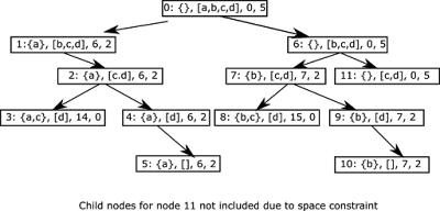
Modeling this in a binary tree we will get a tree looking like this. Each node is numbered.

You can see from the above diagram that each node has the four features outlined above in order. For Node 0, the root, the set of items that are taken are the empty set, the list of items to make a decision is all the items, the total value of items taken is 0, and the remaining space in the knapsack is 5. At the next level, when we choose item ‘a’, the quadruple changes in node 1. We chose the left branch, node 1, because the weight of item ‘a’, 3, is less than the remaining space which is 5. Choosing the left branch, item ‘a’, then reduces the available space to 2, and changes the other items for that node. The right branch to the root node is node 6 which involves the decision not to choose item ‘a’. If we decide not to choose item ‘a’ but remove it from the list, then we see that the set of items taken remain empty, the list of items has reduced to only [b,c,d], the total value of items taken is still 0 and the remaining space is still 5. We do this decision structure, making the decision to choose or not to choose an item and updating the node accordingly until we get to a leaf node.

Characteristics of a leaf node in our graph: a leaf node is a node that either has the list of items not taken to be empty, or the remaining space in knapsack to be 0. Note this because we will reflect this when writing our recursive algorithm.

Now, this problem has overlapping sub-problems and optimal substructures which are features any problem that can be solved with dynamic programming should have. We will refer to the graph above in enumerating these two facts.

Overlapping sub-problems: If you look at each level, you will notice that the list of items to be taken for each level is the same. For example in level 1 for both the left and right branch from the root node, the list of items to be taken is [b,c,d] and each node depends on the list of items to be taken as well as the remaining weight. So, if we can find a solution for the list of items to be taken at each level, and store the result (remember memoization) we could reuse this result anytime we encounter that same list of items in the recursive solution.

Optimal substructure: If you look at the graph, you can see that the solutions to nodes 3 and 4 combine to give the solution for node 2. Likewise, the solutions for nodes 8 and 9 combine to give the solutions for node 7. And each of the sub-problems have their own optimal solutions that would be combined. So, the binary tree representation has optimal substructure.

Noting that this problem has overlapping sub-problems and an optimal substructure, this will help us to now write an algorithm using memoization technique for the knapsack problem. If you want a refresher on the dynamic programming paradigm with memoization, see this blog post which I have earlier referenced.

So, we will take a pass at the code for the technique, using the 4 items outlined above. We will be using a knapsack with a weight of 5kg as the maximal capacity of the knapsack. Run the code below to see how it works. I will explain the relevant parts later.

Now let me explain the relevant parts of the code.

Lines 1 – 20: We created the items class with attributes name, value, and weight. Then a __str__() method so we can print each item that is taken.

Lines 22 – 52: This is the main code that implements the dynamic programming paradigm for the knapsack problem. The name of the function is fast_max_val and it accepts three arguments: to_consider, avail, and a dictionary, memo, which is empty by default. To_consider is the list of items that are yet to be considered or that are pending. Remember, this list is what creates our overlapping sub-problems feature along with the avail variable which refers to the weight remaining in the knapsack. The code uses a recursive technique with memoization implementing this as a decision control structure of if elif else statements. The first if statement checks to see that when we come to a node if the pair of ‘length of items to consider’ and ‘weight remaining’ are in the dictionary. If in the dictionary, memo, this tuple is stated to be the result for that node. If not, we move to the next elif statement, lines 30-31 which checks whether this is a leaf node. If this is a leaf node, then either the list of items to consider is empty or the remaining weight is zero (knapsack full), so we say the node is an empty tuple and assign it to result. Then the next elif statement considers the area of branching. Notice from the graph above that the decision tree involves a left branch (take the next item if weight is within limits) and a right branch (don’t take the next item). This elif statement considers the fact where the left branch is not approached and only the right branch. That means for that level, the right node is the optimal result for our parent node. What we do here is call the fast_max_val function recursively to check for child nodes and store the final result as tuples. Then finally, the last else statement. This considers the case where the two branches can be approached. It recursively calls the child nodes of the branches and stores the final optimal result in the variables with_val and with_to_take for the left branch and without_val and without_to_take for the right branch. Then it evaluates which of these two values has the highest value (remembering we are looking for the highest value in each parent node) and assigns that branch to the result.

After the recursion is complete for each node, it stores the result in our dictionary, before calling for any other recursion. Storing this in dictionary is to ensure that when a similar subproblem is encountered, we already have a solution to that problem, thereby reducing the recursive calls for each node.

Finally, the function returns the result as a tuple of optimal values and list of items that were taken.

Lines 55-66: This lines contains the items builder code. It builds the items and then calls the dynamic programming function. Finally when the function returns, it prints out the items that were taken for the optimal solution to the knapsack problem.

If you would like the code to look at it in-depth and maybe run it on your machine, you can download it here.

Now, the beauty of dynamic programming is that it makes recursion scale to high numbers. I want to show that this is possible with the knapsack problem.

I provide another code that implements a random items generator. The test code uses 250 items generated randomly. You can try it on higher number of random items with random values and weights.

The explanation for the codes is similar to the smaller sample above. If you want to take an in-depth look at the code for the higher number of random items, you can download it here.

Happy pythoning.

First Pain-Sensing Electronic Skin that Reacts Like Human Skin

Imagine that you touch a hot stove, how do you perceive that the stove is hot and that you should withdraw your hand? In other words, how did you feel the pain? Doctors tell us that when the skin comes in contact with a hot object such as a hot stove, sensory receptors transfer the information to the nerve fibers at the skin, then the nerve fibers transfer it to the spinal cord and the brainstem where it is then taken to the brain and the information is registered and processed. The brain tells the skin that it has come in contact with a hot object, which then perceives the pain. All of these processes occur in microseconds, Can humans mimic this process with technology?

 

Some scientists at the RMIT University in Australia have concluded that they can mimic the pain reception process of the human skin using an electronic skin. They have built a prototype device that can replicate the way the human skin actually perceives pain and gathers information from the environment. When tested it was found that the reaction of the electronic skin was near instant, close to the instant feedback mechanism we get from our human skin. That is just wonderful.

The team at the university did not just stop there; they went further. They have built stretchable electronic devices that complement the pain reception of the prototype electronic skin which stretchable devices can also sense temperature and pressure. With this accomplishment they have integrated all these functionalities into the prototype electronic skin so that it cannot only perceive pain, it can also perceive temperature and pressure.

Lead researcher, Professor Madhu Bhaskaran, co-leader of the Functional Materials and Microsystems group at RMIT, said that this electronic skin was optimized to act as the human skin.

How the electronic skin works

This optimized electronic skin was a brain child of 3 previous devices and patents that were produced by the team. These patents were:

1. A stretchable electronic device that was transparent and unbreakable. It was made of silicon and could be worn on the skin.

2. Temperature-reactive coatings which are thinner than human hair and could react to changes in the temperature of the surroundings. The coatings were also transformable in the presence of heat.

3. A brain-mimicking electronic device that works as the brain does in using long-term memory to recall and retain previous information.

In the electronic skin prototype, the pressure sensor makes use of the stretchable electronic device and brain mimicking device, the heat sensor makes use of the temperature reactive coatings and the brain-mimicking device using memory cells, while the pain sensor combines all three technologies into one.

PhD researcher Md Ataur Rahman said the memory cells in each prototype were responsible for triggering a response when the pressure, heat or pain reached a set threshold. He hailed this as an accomplishment; the creation of the first electronic somatosensory device that will be able to replicate the complex neural mechanisms involved in transferring information from the skin to the brain and back to the skin in order to interpret what information the skin receptors were receiving from the environment. Compared to previous receptors for the skin which concentrated only on pain, he said this prototype electronic skin was the first of its kind to react to real mechanical pressure, temperature and pain at the same time and provide the correct response.

And this comes with a distinction in reception of different threshold of pain, temperature and pressure.

“It means our artificial skin knows the difference between gently touching a pin with your finger or accidentally stabbing yourself with it – a critical distinction that has never been achieved before electronically,” he said.

A purview of good things to come in the future

According to Bhaskaran: ““It’s a critical step forward in the future development of the sophisticated feedback systems that we need to deliver truly smart prosthetics and intelligent robotics.”

Yes, Imagine a prosthetic leg that could be able to feel real pain, pressure and temperature or even a robot that can distinguish different stimuli. Yes, imagine the future where human creativity has met the demands of Mother Nature. Lead researcher Professor Madhu Bhaskaran said the pain-sensing prototype was a significant advance towards next-generation biomedical technologies and intelligent robotics. We cannot wait to have people without legs know that they can have real legs right now and not feel disadvantaged. Imagine skin grafts that make you feel like this is the real thing and not an artificial skin.

The benefits of this technology are enormous. That is why I decided to include it in my solvingit? blog.

The research was supported by the Australian Research Council and undertaken at RMIT’s state-of-the-art Micro Nano Research Facility for micro/nano-fabrication and device prototyping.

‘Artificial Somatosensors: Feedback receptors for electronic skins’, in collaboration with the National Institute of Cardiovascular Diseases (Bangladesh), is published in Advanced Intelligent Systems (DOI: 10.1002/aisy.202000094).

Python Pow() function For Python Power

The python pow() function, most times called python power function, is a built-in function for calculating the power of a number when raised to an exponent. It comes in very handy several times while doing mathematical operations.

 

The syntax of the python power function is pow(base, exp[, mod]) where base is the number whose power you are looking for, exp is the exponent to which you will raise the base or number, and the optional mod is a modulus integer you might wish to use for the result. In simple terms, it returns the base to the power of the exp.

This is a very simple function to use. In fact, it is one of the simplest I have found in the built-in python functions.

Let’s illustrate its usage with examples.

1. When base is positive and exp is positive.

This is simply the act of raising the base, or number, to the exponent, exp. In literal terms, base ** exp. Consider the example below:

The base is 4 and the exponent is 2. So 4 raised to power 2 gives 16. Very easy to read.

2. When base is negative and the exp is positive.

This is similar to the above. Just raise the base to the exponent.

3. When base is positive or negative but the exponent is negative.

In this case, when the exponent is negative, the result is no longer an int type but a floating point type. Note this difference.

This is correspondent to when you are raising fractions by an exponent. That is why I so love python. You can use it to do so many different things. It gives just the right results for any calculation you assign to it.

4. When you use it with the three arguments, pow(base, exp, mod)

When you use the third optional argument, mod, which means modulus, you are doing an operation which takes the modulus of the result from raising the base by the exponent. Let us illustrate with some examples:

In the above code this is what is happening. The pow() function first raises 4 to the power of 2, the exponent. The result is 16. Then it does 16 modulus 5 which is 1. That’s it.

Do you know that you can even do the modulus of fractional results? Yes, this function gives you the power to do that. Let’s illustrate by raising 4 by negative 2, -2, and get the modulus by 5.

    
base = 4
exp = -2
modulus = 5
n = pow(base, exp, modulus)
print(n)

This new power was introduced in python 3.8. The embedded python interpreter is upgraded only to python 3.6. So, you can run it on your machine and see that 4 raised to the power of negative 2, -2, is 0.0625 and when modulus 5 is called on the result it gives 1.

That’s it. I had a swell time introducing you to this powerful python power function. Play and use it to your heart’s delight. Leave a comment about your findings. I would love to see some comments about this powerful function.

Happy pythoning.

Parsing HTML Using Python

HTML, also known as Hypertext Markup Language, is used for creating web pages and is a standard markup language. If you have ever seen the code of any website or blog, you most probably was reading the HTML code of the page. In this post, we want to parse some HTML strings. By parsing, I mean analyzing the strings syntactically for specific symbols based on the components in the string.

 

We will be using the python class HTMLParser that is contained in the module html.parser for this activity.

All instances or objects of the HTMLParser class are able to parse the markup of text that contains HTML and identify the tags and references that are contained in the text.

To use the HTMLParser class we need to first import it from html.parser module like this: from html.parser import HTMLParser. After that, any user has to inherit from the HTMLParser class and then override any method he desires to use.

But before we start showing that in code, I will first describe some of the methods of the HTMLParser class we will be overriding.

Methods of the HTMLParser class

The HTMLParser class has several methods which are divided into methods that belong to every instance of the class and methods that are called when HTML markup is encountered.

1. Methods of HTMLParser instance.

The two methods that are of interest to us for this post are the HTMLParser.feed() method and HTMLParser.close() method.

The HTMLParser.feed method has the syntax HTMLParser.feed(data) where the data is the text containing markup you want to parse. Processing takes place provided there are complete elements in data and the data is buffered when incomplete until the close() method is called.

The HTMLParser.close method processes all data as if the end-of-file marker has been encountered, thereby closing processing. This method can be redefined in user defined classes but when redefined, it must also be called again.

So, that’s it. Let’s move on to the methods that are used for handling encountered markup.

2. Methods for operating on HTML markup.

The HTMLParser class has several methods for operating on HTML markup, but I will deliberate on only those of interest in the code I will be writing in this blog. They are the common ones. When you know the basics, you can apply other methods to your choosing.

The methods are:

a. Method to handle start tags.

The syntax for this method is HTMLParser.handle_starttag(tag, attrs) and when a start tag in the markup is encountered, it is called with the tag and its corresponding attributes as arguments. So, in your handler code you can directly reference the tag. The attributes are denoted as a tuple of name, value like (name,value) enclosed in a list. So, you can use your for loop or any other method to extract the items in the tuple.

b. Method to handle end tags.

The syntax is HTMLParser.handle_endtag(tag) and the tag is always converted to lower case when markup is encountered.

c. Method to handle tags that have no corresponding end tags, or empty tags.

There are some HTML tags that do not have corresponding end tags like the <br \> tag. This method is designed to handle those. These tags are styled like in XHTML. The syntax for the method is HTMLParser.handle_startendtag(tag, attrs). The structure of the tags and attributes arguments are similar to that of the method to handle start tags.

d. Method to handle comments.

HTML markup contain comments which can be parsed. This method is used to handle them. The syntax is HTMLParser.handle_comment(data) where data is any text that is contained within the <!—Data --> comment.

e. Method to handle data between tags

When you have text that have to be rendered that exist between start and end tags, this method is used to handle those text. The syntax is HTMLParser.handle_data(data) where data is the text that is contained in between start and end tags.

Now that the methods are outlined, let me show how to apply them.

Let’s write a simple code that handles start and end tags when they are encountered, as well as tags that do not have corresponding end tags, or empty tags. The code will ignore comments when encountered in the markup. You can run the code to see the output.

Let me explain relevant parts of the code based on their lines. On line 1 I imported HTMLParser and then on line 3 I created a class, MyHtmlParser, that inherits from HTMLParser. Then inside the class I overrode the methods to handle start tags, empty tags, and end tags, along with comments. For the comments methods, I told the code to ignore all comments. For the end tag handler, I just printed the name of the end tag but preceded by the text, End. For the start tag and empty tags, I first printed out the tag and then printed out the attributes and value, taking a cue from the fact that the attribute and values are stored as pair of tuples.

That’s it. The driver code starts from lines 30 to 35 where I created an instance of MyHtmlParser class called parser and then fed the instance the html text in the variable, text, through the instance’s feed method.

That code was cool but plain simple.

Let’s take another simple code. This time a code that would count the tags and their frequencies in a markup. This promises to be more cool. Just run it to see how it goes.

This time in the code, since we are counting tags, we leave out the end tags handler since when we have identified a start tag that is enough so as not to double count. What the code does is that when any tag is identified, it checks to see if it is in the dictionary, parser_dict, and if it is not in it, it adds it and increments the count by 1 but if it is already in the dictionary, it only increments the count by 1. Just cool.

I hope you enjoyed my code for today. I promise to be bringing you more interesting code that shows how python works and how you can use python to its fullest. Just subscribe to the blog to get updates.

Happy pythoning.

Dynamic Programming In Python: Using Fibonacci Sequence

Dynamic programming is a programming method that aims to optimize solutions to problems. It was developed by Richard Bellman in the 1950s and has since become popular. In dynamic programming, we aim to break down a complicated bigger problem into simpler sub-problems in a recursive manner. If in breaking down the problem into sub-problems we encounter those sub-problems again, the problem is said to be overlapping. Then we try to find the optimal solutions to the sub-problems which solutions will then be combined with other sub-problems to get the overall solution. Thereby, the problem is said to have an optimal substructure.

 

Most times when we have solved the smaller sub-problems we store the results of the solution so that when similar sub-problems are encountered, the results can be reused. This concept in dynamic programming is called memoization. Memoization not only speeds up computing, it also saves on computer resources.

In dynamic programming, we will be using the memoization technique a lot.

To illustrate how dynamic programming is used in practice let us take a problem that has both overlapping sub-problems and an optimal substructure. That is the problem of finding the Fibonacci sequence. We will be using the Fibonacci sequence as an example of dynamic programming in python.

The first ten Fibonacci sequence are: 0, 1, 1, 2, 3, 5, 8, 13, 21, 34. Each item in the sequence is derived from the sum of the two previous items except for the case when n is 0 or 1. Then in those instances, when n is 0 the sequence is 0 and when 1 the sequence is 1.

Traditionally, the Fibonacci sequence can simply be solved using a recursive algorithm. Just like the one below:

In the code, lines 4 and 5 are used to state the cases where n is either 0 or 1. Then if n is neither of these, then recursively we call the sum of the previous two Fibonacci numbers.

This solution or algorithm is simple but not elegant. This is because the complexity of the algorithm is exponential. Therefore, it does not scale for large Fibonacci numbers. If you call it on n being 120, it would take more than 250,000 years to finish. Quite some age. Therefore, it would do with some optimization.

Now, let’s see how dynamic programming with python can help.

First, we state that dynamic programming will be applicable when a problem has overlapping sub-problems and that each sub-problem has an optimal solution which will be combined to give the overall solution. That is what we are doing in the above recursive calls. Let’s illustrate it with some pictures. For example when we are looking for the Fibonacci of 6. Look at the number of calls that are generated.

Each call is a sub-problem. You can see that fib 2 was called 5 times while fib 3 was called 3 times before getting the final result. Since we can generate solution for each of the sub-problems, it would be nice to just generate the solution once, an optimal solution for the sub-problem, and use that result for every time that sub-problem was called. The operation of storing this result and using it for subsequent sub-problems is called memoization. Creating a memo of previously encountered problems that was solved.

Using this concept, we can now write a second code for the Fibonacci sequence based on dynamic programming using python.

As you can see from the dynamic programming code above, we are using memoization with a dictionary, fib_dict, to store already known results of sub-problems and these results are called when similar sub-problems are encountered. In line 9 we created the dictionary and gave it the initial values of the Fibonacci sequence. Then in line 11 we called the Fibonacci function, fast_fib. Lines 1 to 7 contains the code for the Fibonacci computing function, fast_fib. In the code, we first check to see if the key, n, is already in the dictionary, if it is, we return it but if it is not we compute the Fibonacci sequence recursively and store the result so that it can be used in subsequent calls. This is done consecutively as any n is needed. Finally, it returns the value for the key, n, in the dictionary where n is the Fibonacci number we are looking for.

This dynamic programming implementation runs in linear time and it scales considerably. I just so love it. It is much better than the earlier recursive Fibonacci code.

I hope you now know how dynamic programming works and how to implement it in other problem spaces.

Happy pythoning.